DINOv3

The underlying idea behind the advancements of DINOv3 is simple, and this is beautiful. Occam’s Razor is always present and guides daily decisions. So, today you will join me on an exciting path toward learning a simple additional (and fundamental) block of the computer vision.

For those who are not familiar with the self-supervised learning (SSL) field, there will be a super-quick recap as the first chapter. However I’m preparing a super dense and rich post that will be published later.

Let’s dive in and demystify DINOv3!

How to learn by yourself (SSL quick recap)

Self-supervised learning was developed to eliminate (or at least avoid) the expensive and time consuming activity of manual annotation of fully supervised samples.

SSL works as follows:

1. take a big amount of raw data (i.e. a lot of images)
2. choose a pretext task to let the samples themselve be self-explanatory
3. pre-train a model using the pretext task

this paradigm is fundamentally different from supervised learning, where you need to optimize the model to predict, for example, the right classification of the label of an image.

A pretext task is a task inferred from the image itself, that let the model learn the feature of the image. Some examples for image-based datasets are:

• Image rotation: the model must learn if the input image is rotated by 0/90/180/270 degrees.
• Jigsaw puzzle: an image will be divided into a padded grid of 9 patches, and the model must reorder them
• Image inpainting: a piece of the image (i.e. a square) is removed from the original sample, and the model must learn to reconstruct it
• Relative patch location: similar to Jigsaw puzzle, predict the location of a single patch image with respect to another

An important point of the SSL, is that we do not have to monitor the performances against the pretext task used to pretrain the model. What we must do is measure the performance against a selected downstream task like classification and segmentation, after the pretraining using a specific pretext task.

Citing the authors: “Models trained with SSL exhibit additional desirable properties: they are robust to input distribution shifts, provide strong global and local features, and generate rich embeddings that facilitate physical scene understanding.”

DINOv3 ( )

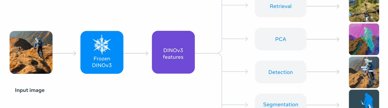
First of all, we are talking about a model which output super-damn-giga-rich features, and is domain- and task- horizontal. To do so, they had to build a single, reusable foundation model.

Well Self-Supervised learning is really helpful in these scenarios because you are making a model learn without even explicit the labels, but inferring them from the data itself. There are also other methodologies (of course) like fully- and weakly- supervised pretraining, but they requires high-quality metadata, and this is of course time-consuming and expensive.

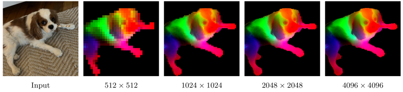first three DinoV3 PCA components computed over three RGB channels.

Well, as we mentioned SSL is not perfect; however, addressing:

1. collection of useful data from unlabeled collections
2. a priori knowledge of optimization horizon on large corpora
3. decrement of the feature’s performances on early training

DINOv3 becomes the universal visual encoder, achieving SOTA performances on downstream tasks.

What it optimizes

There are three components of the learning objective:

1. $\mathcal L_\text{DINO}$: a image-level objective for global alignment [DINO, 2021]

This is the cross-entropy loss between the features extracted from a student ($p_s$) and a teacher ($p_t$) network; both coming from the CLS token of a ViT, obtained from different crops of the same image.

1. $\mathcal L_\text{iBOT}$: a patch-level latent reconstruction [iBOT, 2022]

Some input patches given to the student are getting masked.
Doing so, the authors then apply:

• the “student iBOT” head to the student mask tokens, and
• the “teacher iBOT” head to the teacher patch tokens corresponding to the ones masked in the student

an then, the softmax.

1. $\mathcal L_\text{Koleo}$: a regularizer to spread features uniformly in the space within a batch [KoLeo, 2019]

It comes from the differential entropy estimator; given a set of $n$ vectors (the features) $(x_1,\dots,x_n)$, the $d_{n,i}=\min_{j\ne i}\Vert x_i-x_j\Vert$ is the minimum distance between $x_i$ and any other point within the batch. Then there will be a $l_2$-normalization before the regularizer computation. Spreading out features make them well-separated from other in embedding space, reducing reduncancy, avoiding collapse (all features look alike), and encurange the model to learn meaningful and diverse representations. When this happens, the downstream tasks become easier and more accurate.

All together, are the building block of the DINOv3 loss function:

\[\mathcal L_\text{Pre}=\underbrace{-\sum p_t \log p_s}_{\mathcal L_\text{DINO}} \quad \underbrace{- \sum_i p_{ti}\log p_{si}}_{\mathcal L_\text{iBOT}} \quad \underbrace{- \frac{1}{n}\sum_{i=1}^n \log(d_{n,i})}_{\mathcal L_\text{Koleo}}\]

Underlying model architecture

Scaling law always kicks in

The authors decided that scaling the model is still an option to bring improvements; in fact, from the v2 they increased of $\sim 6$ times the parameter of the ViT. DINOv3 uses ViT 7B (6.7B params) in contrast of the ViT-giant (1.1B) of DINOv2.

How to encode position

They employed a custom variant of the RoPE (Rotary Positional Embedding), first of all they give to each patch a coordinate in a normalized interval $[-1, 1]$; meaning that each patch is within a normalized box.

Using these normalized coordinates (RoPE-box coordinates), for each pair of patches they compute a relative positional bias which will then added to the attention scores. This should help in making the attention mechanism sensitive to how far apart (and in what direction) two patches are situated in the grid.

However, the model should be robust to multiple scales and aspect ratios. To deal with that, they employ a RoPE-box jittering. TO make it simple, instead of using as normalization interval $[-1, 1]$, the authors chose a random value $s\in[0.5, 2]$, perturbing the positional coordinates. Doing so, the normalized coordinates will fall within the interval $[-s, s]$.

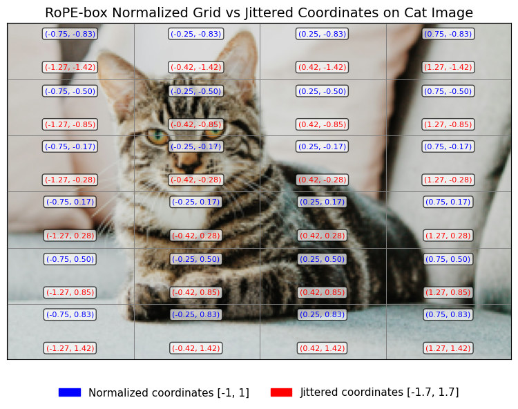A cat image divided into patches. Blue: normalized positions. Red: jittered (scaled) positions. RoPE-box assigns each patch coordinates; jittering augments these, making models robust to scale/aspect changes.

Lowering the number of hyperparams

The idea is the following: when you have a huge model with a gigantic dataset, assessing the optimization horizon a priori is nearly impossible; you should be able to interpret the interplay between, citing the authors, “model capacity and training data complexity”.

Well, the model capacity term is actually an abstract and informal way to indicate how the model is able to learn from more data. You should expect that a model with higher capacity is able to learn more relationships between an higher number of variables.

While the data complexity is simply the combined effects of volume and variety of data.

But why so? With such assumption they are able to train with constant learning rate, weight decay and teacher EMA (Exponential Moving Average) momentum, dropping all scheduling parameters. By doing so they can:

1. train until the downstream task performance continues to improve
2. simplify the hyperparameter choice

The game changer: Gram Anchoring

They had to choose between:

1. almost infinite performance improvement on global benchmarks (e.g. classification)
2. degradation of performance in dense tasks (e.g. segmentation)

Initially they found out that the model could potentially train indefinitely, until the former phenomenon emerged. The extended training arise some patch-level inconsistencies in feature representations, and this undermines the interest of researches in pursuing such direction.

Patch-level inconsistencies

They refers to the gradual (iter-by-iter) degradation in the model’s ability to maintain consistent and meaningful representations for individual image patches as training progress for extended duration.

Explained simply, as the model is trained longer, features for individual patches become less “local”, i.e. their “meaning” do not reflect the underlying content. This can be easily visualized using patch similarity maps.

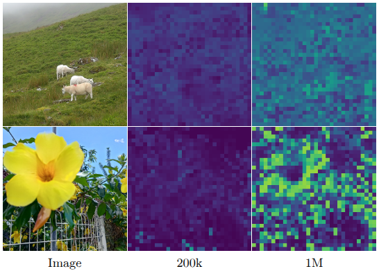
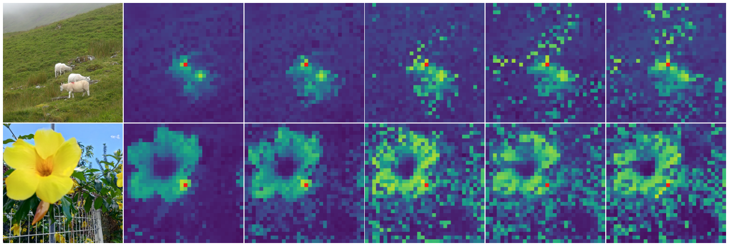Patch similarity (without Gram Anchoring) over iterations.

These maps track how similar each patch’s feature vector of an image is to a reference patch. In early training these similarities are clear and localized; over time become noisy, with many irrelevant patches showing high similarity.

The reason is that the output of the patch, is increasingly (over time) aligned with the global class CLS token, which is the global vector which represent the whole image.

In ViT, the CLS token is a learnable vector that aggregates information from all patches, and is used in global tasks. This settings of Self-Supervised learning make the model learn by optimizing the CLS token. Without additional constraints, this scenario makes the patch features mimic the global vector behavior when training continues. This reduces the ability of the model to distinguish between different patches, because they tend to align with a global class token, so eroding the locality of the patches.

The loss of patch-level consistency is correlated to performance degradation for dense tasks, because they require to have each patch with a distinct meaningful representation to correctly label each region of the image.

Cosine similarities between the `CLS` and output patches.

Gram Anchoring

From the lack of correlation between global and dense performance, there is a relative independence between learning strong discriminative features and maintaining local consistency.

The combination of $\mathcal L_{\text{DINO}}$ with local $\mathcal L_{\text{iBOT}}$ started to address this problem, but the global representation dominates as training progress further.

Gram Anchoring loss is introduced to mitigate the degradation of patch-level consistency without impacting the features. It takes the name from the Gram matrix, which is the matrix of all pairwise dot products of patch features in an image, it capture the spatial correlations, but not the features themselves.

The loss pushes the student Gram matrix toward the one of the Gram teacher, which is an earlier model selected by an early iteration of the teacher network, exhibiting better properties for dense scenarios.

Operating on the Gram matrix (i.e. on the structure of the similarities), the local features can evolve and change as long as the pattern of patchwise relationship remains consistent. Doing so, the model can improve in global tasks and adapt locally while presenting spatial relationships.

The Gram Loss is defined as follows

\[\mathcal L_\text{Gram}=\Vert \mathbf X_S \cdot \mathbf X_S^\top - \mathbf X_G \cdot \mathbf X_G^\top \Vert^2_F\]

where having $P$ as the number of patches of an image and $d$ the dimension at with a network operates, $\mathbf X_S$ ($\mathbf X_G$) is the $P\times d$ matrix of $\mathbf L_2-$normalized local features of the student (teacher).

The authors started applying such matrix after 1M iterations, showing an interesting “repair” behavior of very degraded local features. The gram teacher is getting updated every 10k iterations. This second step of training is called refinement step and it seeks to optimize $\mathcal L_\text{Ref}$

\[\mathcal L_\text{Ref} = w_D\mathcal L_\text{DINO}+\mathcal L_\text{iBOT}+w_\text{DK}\mathcal L_\text{DKoleo}+w_\text{Gram}\mathcal L_\text{Gram}\]

The application of the Gram loss (>1M iterations) display clearly that patch-level consistency is getting repaired with positive impacts on the iBOT loss. In contrast, the global features optimized by the DINO loss, does not get significant modifications.

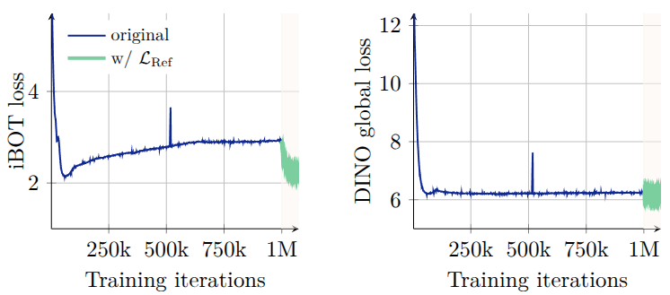Evolution of the patch-level iBOT loss and the global DINO loss.

Conclusions

DINOv3 is a milestone in the field of self-supervised learning revolutionizing the visual representations across multiple domains.

It solves a key problem within long-range training settings, the patch-level consistency, as well as grounding some solid basis for further SSL research, achieving continual global improvement and local (patch-level) feature preservation and enabling robustness in both classification and dense prediction tasks.

References

[DINO, 2021] Caron, Mathilde, et al. “Emerging properties in self-supervised vision transformers.” Proceedings of the IEEE/CVF international conference on computer vision. 2021.

[iBOT, 2022] Zhou, Jinghao, et al. “ibot: Image bert pre-training with online tokenizer.” arXiv preprint arXiv:2111.07832 (2021).

[KoLeo, 2019] Sablayrolles, Alexandre, et al. “Spreading vectors for similarity search.” arXiv preprint arXiv:1806.03198 (2018).