V-JEPA
Features are the most informative parts of a thing, they allows us to understand what we are dealing with. Well, here with V-JEPA, Bardes Et al, tried to leverage them as a stand-alone objective for unsupervised learning (of visual representations from video).
The authors trained V-JEPA solely on feature prediction, this means that unlike other SSL mwthods, which leverages pretrained image encoders, negative examples and hard negatives mining, and a pixel-level reconstruction, V-JEPA relies only on latents.
Let’s go straight to the core.
Video-JEPA
First of all we start by briefly recalling how the Joint-Embedding Predictive Architecture (JEPA) works
 JEPA architecture.
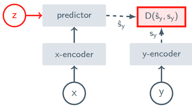
JEPA are trained to predict the representation of an input $y$ from the representation of another input $x$. However, as you can see, there is another variable that comes in play, $z$; it provides to the predictor, informations about the transformation that computes $y$ from $x$.
As an example, imagine a 10 frames long video. Let $y$ be the frame number 8 and $x$ the frame number 2. The model already knows that they are 6 frame apart thanks to the positional encoding, what doesn’t know is what’s happening in the next 6 frames, that yield the video to frame 8.
The variable $z$ helps disambiguating between all possibilities which can occur in such 6 frames of difference, it is the missing information which the predictor needs to correctly try to predict $y$ from $x$.
The basic architecture in comprised of
- a encoder $E_\theta(\cdot)$, which computes the latent representations of the inputs
- a predictor $P_\phi(\cdot)$, which predicts the representation of $y$, from the representation of $x$, conditioned on $z$ (the transformation/corruption between $x$ and $y$)
Multiple scenarios
The author states the following, which in my opinion is worth expanding
Conditioning of $z$ enables the generation of distinct predictions for various transformation of $x$
this may seem a small detail, but instead relies at the core of the JEPA architectures family.
Let me start with a simple, yet effective, example: suppose $x$ is a video of a robot arm approaching a cup, the next frame $y$ could be
- the arm grasping the ucp
- the arm pushing the cup
- the arm missing the cup
if the model tries to predict $y$ from $x$ alone, without knowing which action is getting occurred, the oprimal loss. minimizing strategy is to rpedict an average of all possibilities, which leads to a blurry non-sense ghost arm.
The variabel $z$ acts as a selector/control knob that tells to the predictor which specific transformation or future to generate.
Another example, we have a 60 frames long video about a dog. Let $f_n$ the $n$-th frame of the video with $0\le n\le59$. Let $x=f_0$ the frame number 0 and $y=f_{50}$. Multiple futures are possible between the frame 0 and 50, the dog can
- bark,
- jump,
- roll
the variable $z$ gives to the predictor, the missing causal information needed to correctly predict $y$ from $x$ disambiguating which transformation occurs.
The conditional variable works by saying, for example, that $z=”\text{bark}”$; suggesting the predictor to generate the representation of frame 50 assuming a barking action of the dog.
If $z=”\text{roll}”$ the predictor would yield a different prediction.
Training objective
The visual encoder $E_\theta(\cdot)$ is trained so that the representation of one part of the video $y$ should be predictable from the representation computed from another part of the video $x$.
The predictor network $P_\phi(\cdot)$, which maps $E_\theta(x)$ (the repreentation of $x$) to $E_\theta(y)$ (the representation of $y$), is trained simultaneously with the encoder and is fed with the spatio-temporal positions of $y$ (w.r.t. $x$) through the conditioning variable $z$, also denoted as $\Delta y$.
Having said that, the objective function of Video-JEPA is the following
\[\text{minimize}_{\theta, \phi}\quad \left\Vert P_\phi \left(E_\theta(x),\, z\right)) \;-\; \text{sg}\left(\bar{E}_\theta(y)\right)\right\Vert_1\]well, is not really as clear as you expected, right? You’ll understand in seconds.
Representation collapse
The naive objective is something like this
\[\text{minimize}_{\theta, \phi}\quad \left\Vert P_\phi \left(E_\theta(x),\, z\right)) \;-\; E_\theta(y)\right\Vert_1\]which you can easily read as “minimize the differences between the representation of $y$ and the representation of $x$ conditioned by $z$”. That’s fair, but there is a subtle problem which is hard to spot and easy to overlook.
Ask yourself, which is the trivial solution of this naive objective?
Suppose the encoder (which is shared between $x$ and $y$) start outputting always the very same representation for every single input.
The objective gets minimized, but the network outputs garbage.
This is a well known problem in the SSL literature, which Grill Et al. solved using the BYOL (Bring Your Own Latent) architecture, combining the stop-gradient operation together with the EMA (Exponential Moving Average) updates of the weights of the twin network.
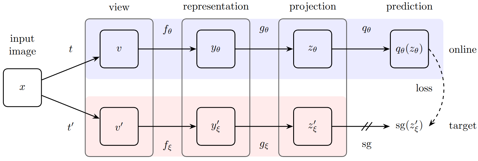 BYOL architecture.
In our case, $\text{sg}(\cdot)$ denote the stop-gradient operation, while $\bar{E}_\theta(\cdot)$ denotes the network with the EMA weights updates.
This should make crystal clear the reasoning behind the non-naive implementation of the objective function.
Inside the paper there is a specific paragraph dedicated to the “Theoretical motivation” for the effectiveness of this collapse prevention strategy.
Prediction task
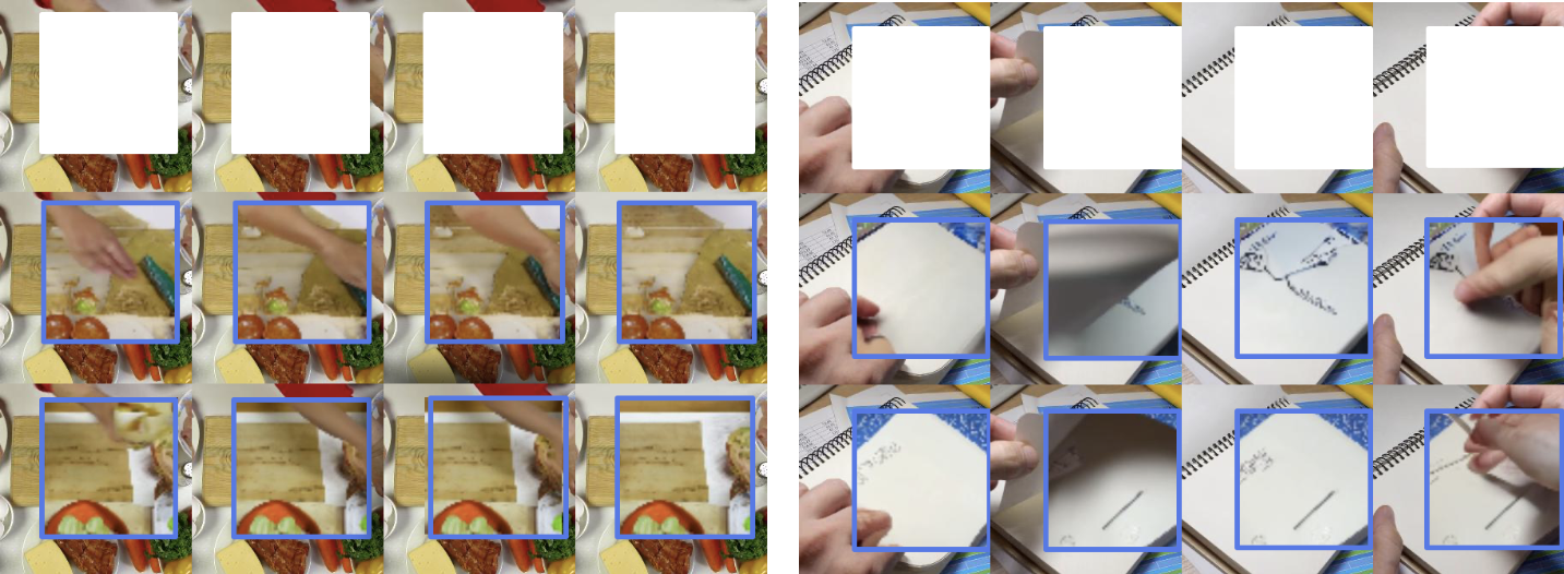
The prediction task is a masked modeling formulation: regions from $x$ and $y$ from the video are samples using masking.
Video data are really “leaky”, since nearby pixels and frames look very similar, and so they are “naturally redundant”. This make the hiding of information inside videos an important part for a correct problem modeling and further training.
To grasp the concept completely, you need to think about the dynamics that can emerge in masking along temporal or spatial dimensions.
Spatial masking
If you hide random pixels, the model easily guess the missing color by looking at pixel right next to it. To avoid so, cutting out large, solid squares or rectangles (i.e. blocks) is the way to proceed.
By removing a whole chunk of a scene, the model must learn to understandthe geometry an the logic of the object for guessing what’s missing, can’t just interpolate colors.
Temporal masking
The temporal dimension also is not really straightforward. If two consecutive frames are block masked in different parts, the model can look to frame 2 and copy information to reconstruct frame 1.
The easiest solution is to take spatial blocks and extend them throughout the temporal dimension (3D blocks) for the entire duration of the clip. In this way, the information is missing for the whole time, so it can’t leverage the “temporal redundancy”.
Masking strategy
The authors leverage two types of masks
- short-range masks: union of 8 randomly sampled blocks ($\sim$ 15% of the frame per block), to force the model learning local context and details
- long-range masks: union of 2 blocks ($\sim$ 70% of the frame per block), to force the model learning global structure
obiouvsly, the blocks can be overlapping. Taking the union of these two masks, the result is that the $\sim$ 90% of the video gets masked, leading the model see only a small part of the context $x$ to predict the target $y$.
It’s worth to mention that the authors performed an ablation study on differentways of masking:
-
random-tube[r], a fraction $r$ of tubes gets removed from $x$ -
causal multi-block[p], restrict $x$ to the first $p$ frames of the 16-frame video -
multi-block, which is the masking strategy described, a random set of spatio-temporal blocks gets masked from $x$.
The multi-block is the masking strategy which performed better.
Predicting Representation vs Pixel
Do we really need that each and every pixel contribute to the loss function, or the representation space is fair enough? Well the answer is easy, and comes directly from the JEPA paper
We conjecture that a crucial component of I-JEPA is that the loss is computed entirely in representation space, thereby giving the target encoder the ability to produce abstract prediction targets, for which irrelevant pixel-level details are eliminated.
however, also in V-JEPA, the authors stated the very same, comparing the feature-level loss with the pixel-level loss.
Evaluation on downstream tasks
Instead of the classical probing mechanism, where to the frozen encoder gets appended a linear classifier, the authors use dthe so-called attentive probing.
It consists of a lightweight trainable module that leverage attention to read out features from the frozen V-JEPA encoder. The Attentive word comes from the usage of a learnable query token; concretely, they do the following
- freeze V-JEPA encoder
- extract feature tokens $s_1, s_2, \dots, s_L$
- introduce a learnable query vector $q$
- compute attention weights using $\text{softmax}(q^\top W_ks_i)$ (the subscript in $W_k$ is not random)
- aggregate features using attention-weighted sum
- feed results to a classifier
that’s it, an attention-based pooling layer.
Why do we need a pooling mechanism?
The V-JEPA encoder outputs many feature tokens which spans across space and time:
- different patches of the frame
- different timesteps
but the final classifier needs one vector.
The baseline to make comparison, is the average pooling, you just treat everything equally; in other words all part of the video are equally important, and this can easily computed as follows
\[y=\dfrac{1}{N}\sum_{i=1}^N s_i\]and this in videos is rarely true since, for example, the background is not always important compared to key motions.
With attentive probing, you do the following
\[y=\dfrac{1}{N}\sum_{i=1}^N \alpha_is_i\]the $\alpha_i$ are the results of the softmax operator mentioned earlier, they comes from a distribution which sums to one; so there are some of them which will weight more then other.
Conclusions
This was the natural extension of JEPA, and the results are awesome. The JEPA paradigm keeps being useful (stay tuned!) as well as the SSL strategies to damp the necessity of supervised labels.
We’ll see in next posts how such paradigm can be applied to perform a huge variety of tasks.
Keep in mind that V-JEPA is, in the end, an encoder which produce features, so the model must be then applied to downstream tasks.
Hove you enjoyes it, stay tuned, a lot of stuffs will come ![]()