Decoding Images: Pills Fourier Transform for 2D & 3D Image Analysis
Today we’ll explore how a classic mathematical tool reveals rich information about patterns, textures, and structures, especially when dealing with noisy or repetitive images.
![]()
Introduction
Fourier transformation are a powerful tools that allows us to write a function in its frequency domain as a sum of a number of sinusoids. Its application domain spans along every engineering and science field. Guess what, Computer Vision is one of the fields in which Fourier Analysis is really helpful.
For example whan dealing with noisy images, or when you need to discover patterns inside an image. We’ll see some of such applications.
Pills of background
The Fourier transform in one dimension is defined as follows: let $f(x)$ be a signal belonging to $\mathbf{R}$
\[\begin{aligned} F(u)&=\int_{-\infty}^{+\infty}f(x)\,e^{-i2\pi u x}dx \end{aligned}\]that can be easily rewritten using the Euler Formula. Here $u$ is the frequency and $F(u)$ is a function lying in Complex domain that carries two important pieces of information:
- Amplitude $A(u)$: that tells you how strong the frequency $u$ is
- Phase $\phi(u)$: that tells you how thw frequency $u$ is shifted in time (or as we’ll see later, in space)
There exists also the inverse mapping, the so called ‘Fourier antitransform’ (or Inverse Fourier transform) and is usefull to reconstruct the original signal
\[f(x)=\int_{-\infty}^{+\infty}F(u)\,e^{i 2\pi u x}du\]the usefulness of such operators lies in the properties they have:
-
we can toogle between time and frequency representations of the signal
-
for every $\omega$ from 0 to $\infty$, $F(\omega)$ maintain both the phase and the amplitude of the input signals
\[A=\pm \sqrt{R(\omega)^2 + I(\omega)^2} \quad \phi = \arctan\dfrac{I(\omega)}{R(\omega)}\] -
in the frequency domain we can extract the amplitude (or frequency) and phase plots, that provides us useful informations
2D settings and the $n$D generalization
The generalization to the 2D domain it’s quite straightforward. Instead of having time signals, we have spatial signals with spatial frequencies and phases. Whatever holds for 1D domain, holds also for 2D domain, but it’s just more verbose (another integral kicks in), here is the 2D Fourier Transform
\[\begin{aligned} F(u, v)=\int_{-\infty}^{+\infty}\int_{-\infty}^{+\infty}f(x, y)\,e^{-i2\pi (ux + vy)}dx\;dy \end{aligned}\]and the usual Antitransform
\[\begin{aligned} f(x, y)=\int_{-\infty}^{+\infty}\int_{-\infty}^{+\infty}F(u, v)\,e^{i2\pi (ux + vy)}du\;dv \end{aligned}\]Being more specific, when we apply fourier transforms to digital images, which are discrite and finite, we can switch to summations in place of the integrals adn we call it Discrete Fourier Transforms (DFT). They are defined as follows
\[\begin{aligned} F(u, v)=\sum_{x=0}^{M-1} \sum_{y=0}^{N-1} f(x, y)\,e^{-i2\pi (\frac{ux}{M} + \frac{vy}{N})}dx\;dy \end{aligned}\]and the antitransform
\[\begin{aligned} f(x, y)=\dfrac{1}{MN}\sum_{u=0}^{M-1} \sum_{v=0}^{N-1} F(u, v)\,e^{i2\pi (\frac{ux}{M} + \frac{vy}{N})}du\;dv \end{aligned}\]Note that from now on I’ll refer to 2D grayscale images, but the very same argument can be applied to RGB images.
Fourier Transforms interpretations
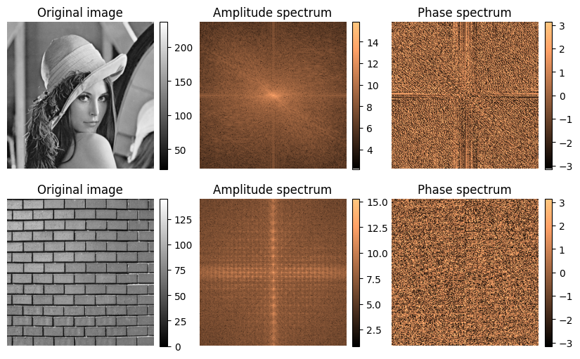
The frequency domain of an image can reveal its textures and periodic patterns, as well as the composition of edges and gradients. In fact, threating an image as a spatial signal, from the frequency domain we obtain its spatial frequencies that encodes meaningful information:
- Low frequencies represent smooth, gradual changes, like the background or large objects
- High frequencies capture sharp edges, fine details and noise
Being signals, they hold also other information: the Magnitude and the Phase of an image encodes a lot of information related to the underlying pixel spatial distribution:
- Magnitude Spectrum indicated how much of each frequency is present.
- Phase Spectrum encoded structural and positional information
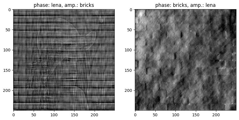
surprisingly the majority of the perceptual structure lies in the phase component: as we’ll see, replacing an image phase while keeping another magniture leads to an hybrid that perceptually looks similar to the phase-donor image.
Example: Lena and the Bricks
The fourier transforms allows us to extract the phase and the plot of an image, and they have the very same meaning we’ve seen in 1D, but here they are spatial:
using logarithmic scale for the amplitude, we obtain the following 3D plot
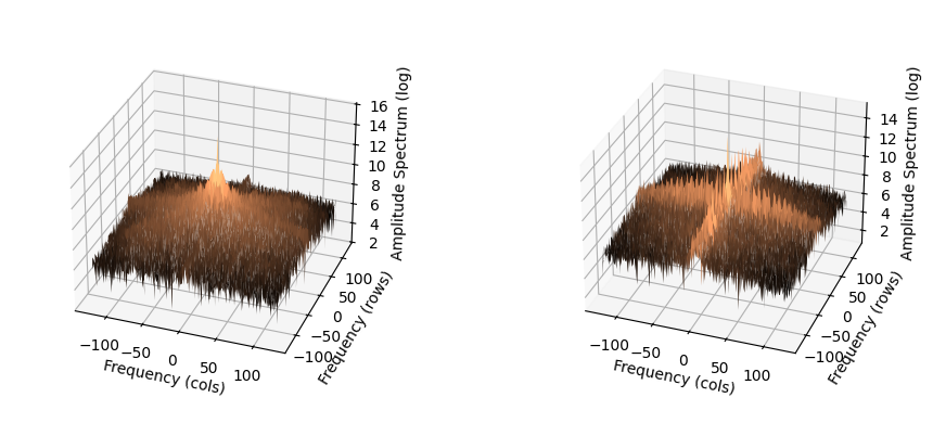
where in the left we have the 3D amplitude spectrum of Lena, while in the right the one for bricks wall (note that is a meshgrid).
Just seeing such results we perceive that these plots gather a lot of informations about the image we are dealing with. A way to handle them is the mixing of amplitude and phase plots from 2 different images
Practical Applications in Images
Image filtering
Using Fourier Transform you can Low-/High-/Band- pass filter the input image. In this way you can remove high frequency components like noise and edges (i.e. blurr the image) using Low-pass filtering, remove low-frequency components enhancing edges and details with the High-pass filtering, and perform a texture analysys and feature extraction by focusing on a specifuc frequency range with the Band-pass filtering.
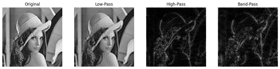
Image Compression
natural images tend to have most of their visual variance (i.e. information, energy) concentrated in low spatial frequencies (smooth gradients, large homogeneous regions) while high frequencies due to fine details carry less energy.
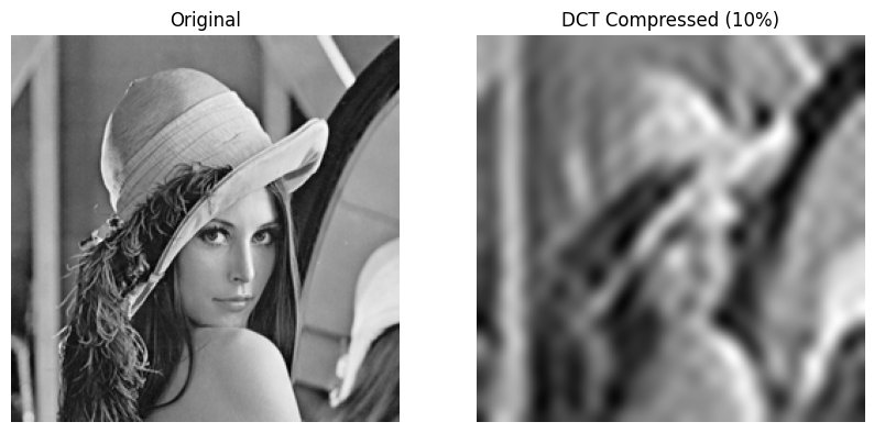
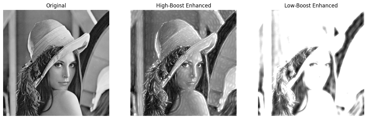
Image Enhancement
in frequency domain, global and local features are separate by frequency band. A way to enhance images uses the so called High-Boost Filtering, which is defined as follows
\[H(u, v)=A+D(u, v)\]with $A>1$ and $D(u,v)$ an high-pass mask. The same holds using a low pass mask.
Watermarking in Frequency Domain
the watermark shoud not be visible under normal viewing (the example has exaggerated watermark strength on purpose). It is capable to survive common signal/image processing techniques (compression, cropping, filtering) and geometric distortions (scaling, rotation). This method is useful to allow embedding reasonable payload securely, resisting to malicious removal. A typical embedding strategy is the Additive Spread Spectrum, which states the following:
\[F_w(u,v)=F(u,v)+\alpha W(u,v)\]where $W$ is a structured pattern and $\alpha$ governs the stength/visibility of the pattern. There are of course also other strategies.
